Step 1: Estimating generalization
Holdout Validation
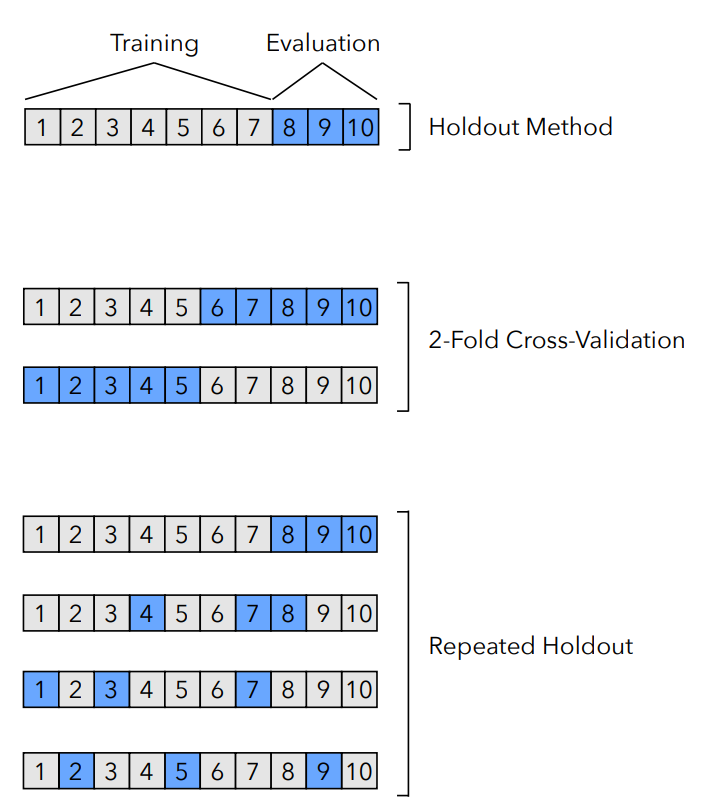
If we train and evaluate our model on the same dataset, we run the risk of overfitting our model, which will introduce an optimistic bias. A very simple way to tackle this problem is to split the data into two non-overlapping sets: the training set and a test set. We could then use the former set for training and the latter set for evaluation. Notice that the test set should only be used once in order to avoid data leakages that may introduce bias.
We illustrate here how holdout validation can be used to estimate the accuracy of our model:
Step 1. Split the data into two non-overlapping subsets: a training and a test set. The training set should be larger than the test set, but it is important to remember that the test set should still be large enough to provide a good estimation. Some common training/test splits are: 23/13. 60/40, 70/30, 80/20 or 90/10.
Step 2. Fit the model
Step 3. Get the predictions of the model on test data and calculate test set accuracy
Step 4 (optional). If we do not need to use the test set in the future, we can then feed the test data to the algorithm for training
Some possible issues with this method:
Resampling violates the assumption of independent, identically distributed samples
Resampling may not give us an accurate representation of the distribution, modifying the statistics of the sample. For example, in a classification task we may end up not having enough samples from one class in the training data.
Having our data split one way may not give us an accurate estimate of the performance of the algorithm.
If the training set is not large enough, the model may not have reached capacity. In this case, reducing the amount of training data may introduce a pessimistic bias.
These are possible ways to mitigate these issues:
Repeated Holdout Validation
A more precise way to evaluate generalization is to repeat the holdout method k times, each time with a different training/test split. The performance could then be estimated as the average over the k repetitions:
Having more than one train/test split can also help us evaluate the stability of the model.
K-fold cross-validation
Another way to have more than one split is to divide the data in k equal parts: one part for validation and the remaining k-1 parts for training. We then iterate this process such that each one of the parts gets to be the validation set. The accuracy is then estimated as the average performance over the k splits. This method is more commonly used for model selection rather than evaluation.
Notice that if we set the number of folds equal to the number of data points, then we have a process called leave-one-out cross-validation. This process is computationally expensive but often employed in small datasets.
Stratification
In some cases, for example in the presence of strong class imbalance, resampling may introduce issues. It could be beneficial to sample the data in a way that maintains the original class ratio in both the training and the test set. This is the preferred method for most applications. An implementation for this method can be found on sklearn.
Bootstrap method
Bootstrapping allows us to estimate a quantity by repeatedly sampling the data. Specifically, bootstrapping performs sampling with replacement, whereas holdout performs sampling without replacement. We illustrate here how bootstrapping can be used to estimate the accuracy of our model:
Step 1. We take the whole dataset of size n
Step 2. For k rounds: We draw n samples with replacement from the original data. This implies that each data point may appear multiple times in one bootstrap sample.
Step 3. For each one of the k bootstrap samples, we fit a model and compute the accuracy.
Step 4. We compute the average accuracy over the k bootstrap samples:
Last updated
